Convolutional Theorem

Important note: this particular section will be expanded upon after the Fourier transform and Fast Fourier Transform (FFT) chapters have been revised.

Now, let me tell you about a bit of computational magic:

Convolutions can be performed with Fourier Transforms!

This is crazy, but it is also incredibly hard to explain, so let me do my best. As described in the chapter on Fourier Transforms, Fourier Transforms allow programmers to move from real space to frequency space. When we transform a wave into frequency space, we can see a single peak in frequency space related to the frequency of that wave. No matter what function we send into a Fourier Transform, the frequency-space image can be interpreted as a series of different waves with a specified frequency. Each of these waves is parameterized by another $e^{2\pi i k n / N}$ term, where $k$ is the element's value in the frequency domain, $n$ is its value in the time domain, and $N$ is the overall length of the signal. In this way, each wave can be seen as a complex exponential.

So here's the idea: if we take two functions $f(x)$ and $g(x)$ and move them to frequency space to be $\hat f(\xi)$ and $\hat g(\xi)$, we can then multiply those two functions and transform them back into to blend the signals together. In this way, we will have a third function that relates the frequency-space images of the two input functions. This is known as the convolution theorem which looks something like this:

$\mathcal{F}(f*g) = \mathcal{F}(f) \cdot \mathcal{F}(g)$

Where $\mathcal{F}$ denotes the Fourier Transform.

At first, this might not seem particularly intuitive, but remember that frequency space is essentially composed of a set of exponentials. As mentioned in the section about Multiplication as a Convolution, multiplication in base 10 space is also a convolution. The convolutional theorem extends this concept into multiplication with any set of exponentials, not just base 10. Obviously, this description is still lacking a bit of explanation, but I promise we will add more when revising the Fourier transform sections!

By using a Fast Fourier Transform (FFT) in code, this can take a standard convolution on two arrays of length $n$, which is an $\mathcal{O}(n^2)$ process, to $\mathcal{O}(n\log(n))$. This means that the convolution theorem is fundamental to creating fast convolutional methods for certain large inputs.

# using the convolutional theorem
function convolve_fft(signal1::Array{T}, signal2::Array{T}) where {T <: Number}
    return ifft(fft(signal1).*fft(signal2))
end

This method also has the added advantage that it will always output an array of the size of your signal; however, if your signals are not of equal size, we need to pad the smaller signal with zeros. Also note that the Fourier Transform is a periodic or cyclic operation, so there are no real edges in this method, instead the arrays "wrap around" to the other side, creating a cyclic convolution like we showed in the periodic boundary condition case for the one-dimensional convolution.

Example Code

For this example code, we will be using two sawtooth functions as we did in the chapter on one-dimensional convolutions:

using FFTW
using LinearAlgebra
using DelimitedFiles

# using the convolutional theorem
function convolve_fft(signal1::Array{T}, signal2::Array{T}) where {T <: Number}
    return ifft(fft(signal1).*fft(signal2))
end

function main()

    # sawtooth functions for x and y
    x = [float(i)/200 for i = 1:200]
    y = [float(i)/200 for i = 1:200]

    # Normalization is not strictly necessary, but good practice
    normalize!(x)
    normalize!(y)

    # cyclic convolution via the convolutional theorem
    fft_output = convolve_fft(x, y)

    # outputting convolutions to different files for plotting in external code
    # note: we are outputting just the real component because the imaginary
    #       component is virtually 0
    writedlm("fft.dat", real(fft_output))

end

main()

from scipy.fft import fft, ifft
import numpy as np

# using the convolutional theorem
def convolve_fft(signal1, signal2):
    return ifft(np.multiply(fft(signal1),fft(signal2)))

# Sawtooth functions
x = [float(i)/200 for i in range(1,101)]
y = [float(i)/200 for i in range(1,101)]

x /= np.linalg.norm(x)
y /= np.linalg.norm(y)

# Convolving the two signals
fft_output = convolve_fft(x, y)

np.savetxt("fft.dat", np.real(fft_output))

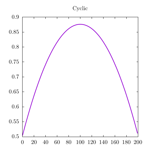
This should produce the following output:

License

Code Examples

The code examples are licensed under the MIT license (found in LICENSE.md).

Images/Graphics

• The image "Cyclic" was created by James Schloss and is licensed under the Creative Commons Attribution-ShareAlike 4.0 International License.

Text

The text of this chapter was written by James Schloss and is licensed under the Creative Commons Attribution-ShareAlike 4.0 International License.

Pull Requests

After initial licensing (#560), the following pull requests have modified the text or graphics of this chapter:

• none