What's a probability distribution?

Probability distributions are mathematical functions that give the probabilities of a range or set of outcomes. These outcomes can be the result of an experiment or procedure, such as tossing a coin or rolling dice. They can also be the result of a physical measurement, such as measuring the temperature of an object, counting how many electrons are spin up, etc. Broadly speaking, we can classify probability distributions into two categories - discrete probability distributions and continuous probability distributions.

Discrete Probability Distributions

It's intuitive for us to understand what a discrete probability distribution is. For example, we understand the outcomes of a coin toss very well, and also that of a dice roll. For a single coin toss, we know that the probability of getting heads $(H)$ is half, or $P(H) = \frac{1}{2}$. Similarly, the probability of getting tails $(T)$ is $P(T) = \frac{1}{2}$. Formally, we can write the probability distribution for such a coin toss as,

$$P(n) = \begin{matrix} \displaystyle \frac 1 2 &;& n \in \left\{H,T\right\}. \end{matrix}$$

Here, $n$ denotes the outcome, and we used the "set notation", $n \in\left\{H,T\right\}$, which means "$n$ belongs to a set containing $H$ and $T$". From the above equation, we can also assume that any other outcome for $n$ (such as landing on an edge) is incredibly unlikely, impossible, or simply "not allowed" (for example, just toss again if it does land on its edge!).

For a probability distribution, it's important to take note of the set of possibilities, or the domain of the distribution. Here, $\left\{H,T\right\}$ is the domain of $P(n)$, telling us that $n$ can only be either $H$ or $T$.

If we use a different system, the outcome $n$ could mean other things. For example, it could be a number like the outcome of a die roll which has the probability distribution,

$$P(n) = \begin{matrix} \displaystyle\frac 1 6 &;& n \in [\![1,6]\!] \end{matrix}.$$ This is saying that the probability of $n$ being a whole number between $1$ and $6$ is $1/6$, and we assume that the probability of getting any other $n$ is $0$. This is a discrete probability function because $n$ is an integer, and thus only takes discrete values.

Both of the above examples are rather boring, because the value of $P(n)$ is the same for all $n$. An example of a discrete probability function where the probability actually depends on $n$, is when $n$ is the sum of numbers on a roll of two dice. In this case, $P(n)$ is different for each $n$ as some possibilities like $n=2$ can happen in only one possible way (by getting a $1$ on both dice), whereas $n=4$ can happen in $3$ ways ($1$ and $3$; or $2$ and $2$; or $3$ and $1$).

The example of rolling two dice is a great case study for how we can construct a probability distribution, since the probability varies and it is not immediately obvious how it varies. So let's go ahead and construct it!

Let's first define the domain of our target $P(n)$. We know that the lowest sum of two dice is $2$ (a $1$ on both dice), so $n \geq 2$ for sure. Similarly, the maximum is the sum of two sixes, or $12$, so $n \leq 12$ also.

So now we know the domain of possibilities, i.e., $n \in [\![2,12]\!]$. Next, we take a very common approach - for each outcome $n$, we count up the number of different ways it can occur. Let's call this number the frequency of $n$, $f(n)$. We already mentioned that there is only one way to get $n=2$, by getting a pair of $1$s. By our definition of the function $f$, this means that $f(2)=1$. For $n=3$, we see that there are two possible ways of getting this outcome: the first die shows a $1$ and the second a $2$, or the first die shows a $2$ and the second a $1$. Thus, $f(3)=2$. If you continue doing this for all $n$, you may see a pattern (homework for the reader!). Once you have all the $f(n)$, we can visualize it by plotting $f(n)$ vs $n$, as shown below.

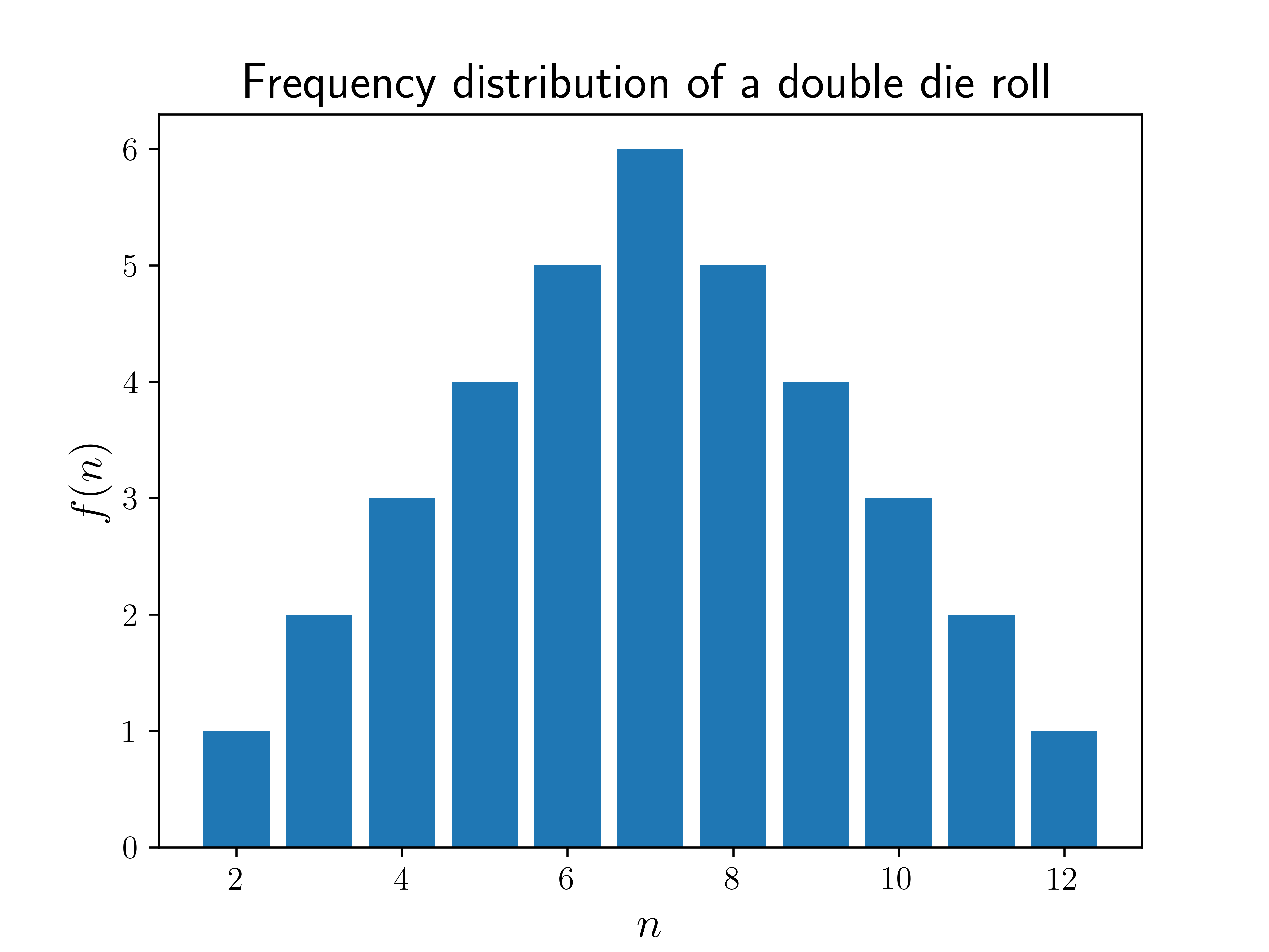
We can see from the plot that the most common outcome for the sum of two dice is a $n=7$, and the further away from $n=7$ you get, the less likely the outcome. Good to know, for a prospective gambler!

Normalization

The $f(n)$ plotted above is technically NOT the probability $P(n)$ – because we know that the sum of all probabilities should be $1$, which clearly isn't the case for $f(n)$. But we can get the probability by dividing $f(n)$ by the total number of possibilities, $N$. For two dice, that is $N = 6 \times 6 = 36$, but we could also express it as the sum of all frequencies,

$$N = \sum_n f(n),$$

which would also equal to $36$ in this case. So, by dividing $f(n)$ by $\sum_n f(n)$ we get our target probability distribution, $P(n)$. This process is called normalization and is crucial for determining almost any probability distribution. So in general, if we have the function $f(n)$, we can get the probability as

$$P(n) = \frac{f(n)}{\displaystyle\sum_{n} f(n)}.$$

Note that $f(n)$ does not necessarily have to be the frequency of $n$ – it could be any function which is proportional to $P(n)$, and the above definition of $P(n)$ would still hold. It's easy to check that the sum is now equal to $1$, since

$$\sum_n P(n) = \frac{\displaystyle\sum_{n}f(n)}{\displaystyle\sum_{n} f(n)} = 1.$$

Once we have the probability function $P(n)$, we can calculate all sorts of probabilites. For example, let's say we want to find the probability that $n$ will be between two integers $a$ and $b$, inclusively (also including $a$ and $b$). For brevity, we will use the notation $\mathbb{P}(a \leq n \leq b)$ to denote this probability. And to calculate it, we simply have to sum up all the probabilities for each value of $n$ in that range, i.e.,

$$\mathbb{P}(a \leq n \leq b) = \sum_{n=a}^{b} P(n).$$

Probability Density Functions

What if instead of a discrete variable $n$, we had a continuous variable $x$, like temperature or weight? In that case, it doesn't make sense to ask what the probability is of $x$ being exactly a particular number – there are infinite possible real numbers, after all, so the probability of $x$ being exactly any one of them is essentially zero! But it does make sense to ask what the probability is that $x$ will be between a certain range of values. For example, one might say that there is $50\%$ chance that the temperature tomorrow at noon will be between $5$ and $15$, or $5\%$ chance that it will be between $16$ and $16.5$. But how do we put all that information, for every possible range, in a single function? The answer is to use a probability density function.

What does that mean? Well, suppose $x$ is a continous quantity, and we have a probability density function, $P(x)$ which looks like

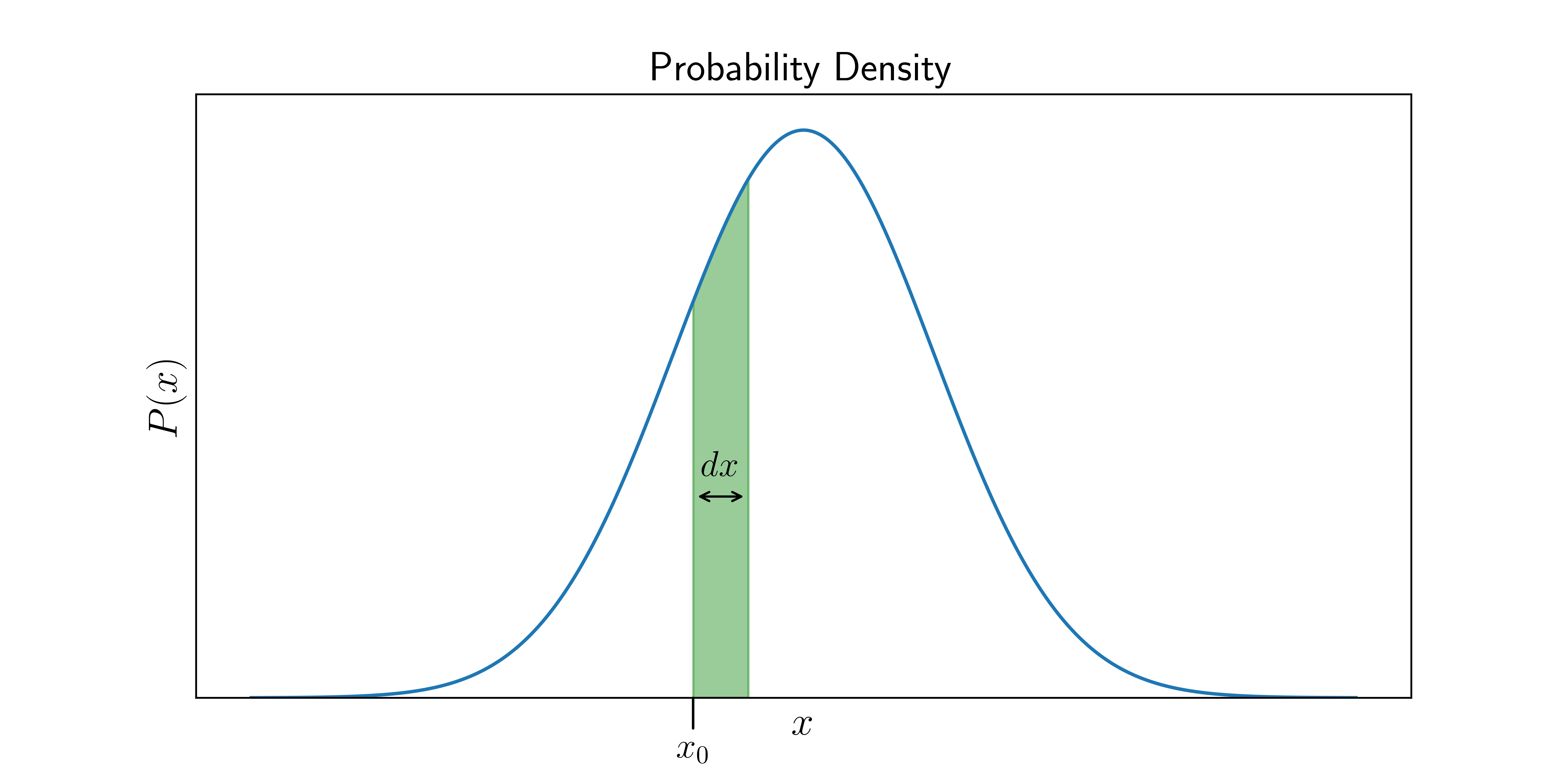
Now, if we are interested in the probability of the range of values that lie between $x_0$ and $x_0 + dx$, all we have to do is calculate the area of the green sliver above. This is the defining feature of a probability density function:

the probability of a range of values is the area of the region under the probability density curve which is within that range.

So if $dx$ is infinitesimally small, then the area of the green sliver becomes $P(x)dx$, and hence,

$$\mathbb{P}(x_0 \leq x \leq x_0 + dx) = P(x)dx.$$

So strictly speaking, $P(x)$ itself is NOT a probability, but rather the probability is the quantity $P(x)dx$, or any area under the curve. That is why we call $P(x)$ the probability density at $x$, while the actual probability is only defined for ranges of $x$.

Thus, to obtain the probability of $x$ lying within a range, we simply integrate $P(x)$ between that range, i.e.,

$$\mathbb{P}(a \leq x \leq b ) = \int_a^b P(x)dx.$$

This is analagous to finding the probability of a range of discrete values from the previous section:

$$\mathbb{P}(a \leq n \leq b) = \sum_{n=a}^{b} P(n).$$

The fact that all probabilities must sum to $1$ translates to

$$\int_D P(x)dx = 1.$$

where $D$ denotes the domain of $P(x)$, i.e., the entire range of possible values of $x$ for which $P(x)$ is defined.

Normalization of a Density Function

Just like in the discrete case, we often first calculate some density or frequency function $f(x)$, which is NOT $P(x)$, but proportional to it. We can get the probability density function by normalizing it in a similar way, except that we integrate instead of sum:

$$P(\mathbf{x}) = \frac{f(\mathbf{x})}{\int_D f(\mathbf{x})d\mathbf{x}}.$$

For example, consider the following Gaussian function (popularly used in normal distributions),

$$f(x) = e^{-x^2},$$

which is defined for all real numbers $x$. We first integrate it (or do a quick google search, as it is rather tricky) to get

$$N = \int_{-\infty}^{\infty} e^{-x^2} dx = \sqrt{\pi}.$$

Now we have a Gaussian probability distribution,

$$P(x) = \frac{1}{N} e^{-x^2} = \frac{1}{\sqrt{\pi}} e^{-x^2}.$$

In general, normalization can allow us to create a probability distribution out of almost any function $f(\mathbf{x})$. There are really only two rules that $f(\mathbf{x})$ must satisfy to be a candidate for a probability density distribution:

1. The integral of $f(\mathbf{x})$ over any subset of $D$ (denoted by $S$) has to be non-negative (it can be zero): $$\int_{S}f(\mathbf{x})d\mathbf{x} \geq 0.$$
2. The following integral must be finite: $$\int_{D} f(\mathbf{x})d\mathbf{x}.$$

License

Images/Graphics

• The image "Frequency distribution of a double die roll" was created by K. Shudipto Amin and is licensed under the Creative Commons Attribution-ShareAlike 4.0 International License.

• The image "Probability Density" was created by K. Shudipto Amin and is licensed under the Creative Commons Attribution-ShareAlike 4.0 International License.

Text

The text of this chapter was written by K. Shudipto Amin and is licensed under the Creative Commons Attribution-ShareAlike 4.0 International License.

Pull Requests

After initial licensing (#560), the following pull requests have modified the text or graphics of this chapter:

• none