The Metropolis Algorithm

The Monte Carlo Integration method uses random numbers to approximate the area of pretty much any shape we choose. The Metropolis algorithm [1] is a slightly more advanced Monte Carlo method which uses random numbers to approximate a probability distribution:

$P(\mathbf{x}) = \frac{f(\mathbf{x})}{\displaystyle\int_D f(\mathbf{x})d\mathbf{x}},$

where $D$ is the domain of $P(\mathbf{x})$ , i.e., all possible values of the $\mathbf{x}$ for which $P(\mathbf{x})$ is defined. $f(\mathbf{x})$ is a function that is proportional to $P(x)$ , such as a statistical frequency distribution which counts the number of occurrences of each $\mathbf{x}$ . The integral in the denominator is the normalization factor which ensures that the sum of all probabilities is unity, i.e., $\int_D P(\mathbf{x}) d\mathbf{x} = 1.$ A one-dimensional example is the normal distribution, or Gaussian distribution, given by

$P(x) = \frac{e^{-x^2}}{\displaystyle\int_{-\infty}^{\infty} e^{-x^2} dx} = \frac{1}{\sqrt{\pi}} e^{-x^2}.$

In practice, it's often easy for us to know $f(x)$ , but the integral in the denominator can be quite difficult to calculate, even numerically. This is especially true when the coordinates ( $\mathbf{x}$ ) are multidimensional, and $f(\mathbf{x})$ is an expensive calculation, as we shall see in the examples below.

An example application

One example of a complicated probability function arises when considering a physical system of $N$ particles. These could be atoms, molecules, or even star systems! For such systems, we can usually describe the potential energy [2] of the system as a function of the coordinates of all particles, $\mathbf{x}$ ,

$E(\mathbf{x}) = E(x_1, y_1, z_1, x_2, y_2, z_2, ... ,x_N, y_N, z_N),$

where $x_i, y_i, z_i$ are the spatial coordinates of particle $i$ . So altogether there are $3N$ coordinates – making $E(\mathbf{x})$ a $3N$ dimensional function, which can be a computationally intensive calculation on it's own. But it doesn't end there!

The physicist Ludwig Boltzmann [3] discovered that when such a system is in equilibrium at some temperature $T$ , you can describe the probability density of the system for any set of coordinates $\mathbf{x}$ using, [4]

$P(\mathbf{x}) = \frac{\displaystyle \exp\left[{\displaystyle\frac{-E(\mathbf{x})}{T} } \right]} {Q},$

where the numerator is called the Boltzmann factor, and $Q$ is the normalization constant,

$Q = \int_D \exp\left[{\displaystyle\frac{-E(\mathbf{x})}{T} } \right] d\mathbf{x}.$

We can see now that the probability density function is a difficult calculation, particularly because of $Q$ . Almost always, no analytical solution exists to the integral in $Q$ , and the numerical integration is unfeasible.

To see that $Q$ is unfeasible to calculate, imagine there are just $10$ particles which all exist in a $1$ D world, restricted to a line segment.

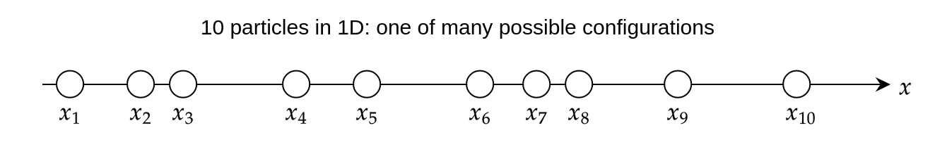
Let's assume that the particles interact, meaning that the position of one particle affects that of another. This could be the case, for example, if all the particles were charged, and so they would be repelling or attracting each other. This means that the energy $E(\mathbf{x}) = E(x_1,...,x_{10})$ of the system is a $10$ D function, and it would not be possible to simplify it any further due to the interactions. Thus, the Boltzmann factor, $\exp\left[-E(\mathbf{x})/T\right]$ , is also a $10$ D function. To calculate $Q$ , we would have to integrate the Boltzmann factor $10$ times, one for each coordinate,

$Q = \int_{x_1} \dots \int_{x_{10}} \exp\left[\frac{-E(x_1,\dots x_{10})}{T}\right]\ dx_1\dots dx_{10}.$

In most cases, there is no known analytical expression for the above integral, so it has to be done numerically. To do so, imagine that we divide the $1$ D line segment into only $50$ different intervals, allowing each particle to take on $50$ different positions. This is equivalent to dividing the length of a football field into intervals of about $2$ meters – not a resolution you'd wanna watch a game in! Even with such poor resolution, the number of different combinations of positions is $10^{50}$ – a colossal number indeed. To see how large this number is, imagine that a single computation of $E(\mathbf{x})$ took only $1$ nanosecond on a single processor, which is much faster than most energy calculations for physical systems in practice. With that speed, it would require $10^{41}$ seconds on a single processor to calculate $Q$ – which means that even with all the processors in the world running in parallel (there could be billions or trillions of them), calculating $Q$ would still take longer than the age of the universe – by many orders of magnitude!

What's really powerful about the Metropolis approach is that you don't need to know the probability function itself. Instead, you just need a function which is proportional to it. What this means for the Boltzmann distribution is that you only need to know the term,

$f(\mathbf{x}) = \exp\left[{\displaystyle\frac{-E(\mathbf{x})}{T} } \right].$

The Metropolis algorithm can bypass the calculation of $Q$ altogether and use $f(x)$ to generate a distribution of $x$ which follows the probability density $P(x)$ . In other words, it can sample values of $x$ in such away that the probability of sampling $x$ will follow the actual distribution $P(x)$ . Thus, if Metropolis was used to sample from $x$ , the number of occurrences of $x$ would be proportional to $P(x)$ . Numerical normalization can then be done by using the total number of samples instead of performing an integration. This fact dramatically reduces the number of calculations needed to approximate the probability distribution.

Finally, the Metropolis algorithm can be modified or implemented in other methods, and forms the basis of many advanced sampling algorithms. The most popular is probably the Metropolis-Hastings algorithm [5] which is fundamentally the same. Some other algorithms that use this method are Metropolis-adjusted Langevin algorithm [6], and Hamiltonian Monte Carlo [7], to name a few. They are often used for physical systems that follow a Boltzmann distribution.

A Random Walk in One Dimension

In the rest of this chapter, we will look at $1$ D examples to understand the Metropolis algorithm. Although the algorithm is not particularly efficient in just one dimension, it is much easier to understand in one dimension than in multiple dimensions. The Metropolis algorithm is very similar to a random walk, so let's first see how we can get a distribution from a random walk.

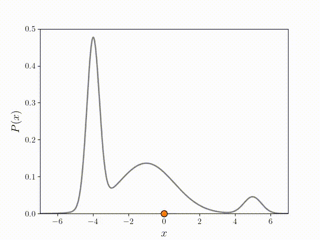
The dot in the figure above is a "walker", whose initial position is $x=0$ . The step size, $g$ , is a random number in the interval $(-1, 1)$ . To get the next position of the walker, we simply generate $g$ and add it to the current position. To get a distribution of $x$ from this walk, we can divide the domain into discrete locations or "bins" and count how often the walker visits each bin. Each time it visits a bin, the frequency for that bin goes up by one. Over many iterations, we get a frequency distribution of $x$ .

A Random Walk With an Acceptance Criterion

The Metropolis algorithm works in a similar way to the random walk, but differs crucially in one way – after choosing a random step for the walker, a decision is made about whether to accept or reject the step based on the function $f(x)$ . To understand how this works, let's call $x_t$ the position before the step, and $x'$ the position after it. We then define the probability of accepting the step to be

$A = \min \left(\frac{f(x')}{f(x_t)}, 1\right).$

The $\min$ function above implies that $A=1$ if $f(x') \gt f(x_t)$ , which means that the move will always be accepted if it is toward a higher probability position. Otherwise, it will be accepted with a probability of $f(x') / f(x_t)$ . If we create a histogram of this walk for some arbitrary target function $P(x)$ , we can see from the figure below that the frequency starts to look very much like it after many iterations!

Although convergence occurs eventually, not all parts of the distribution achieve convergence quickly. Note from the animation above, that the walker very quickly replicates the distribution of the two peaks on the left, but takes quite a while to even reach the third peak to the right. This is because there is a long low probability region between the third peak and second peak that acts as a "barrier." This may not necessarily be a bad thing – sometimes one might want to estimate how long something takes to transition from one state to another, and often these peaks represent such 'states'. So averaging over many metropolis runs may give some estimate of these transition times. If global sampling is the goal, the process of exploration could be sped up by choosing larger step sizes for the walker, for example by choosing step size $g$ from an interval like $(-3,3)$ instead of $(-1,1)$ .

The Algorithm for a One Dimensional Example

Now let's dive into the actual algorithm with some example code!

The Initial Setup

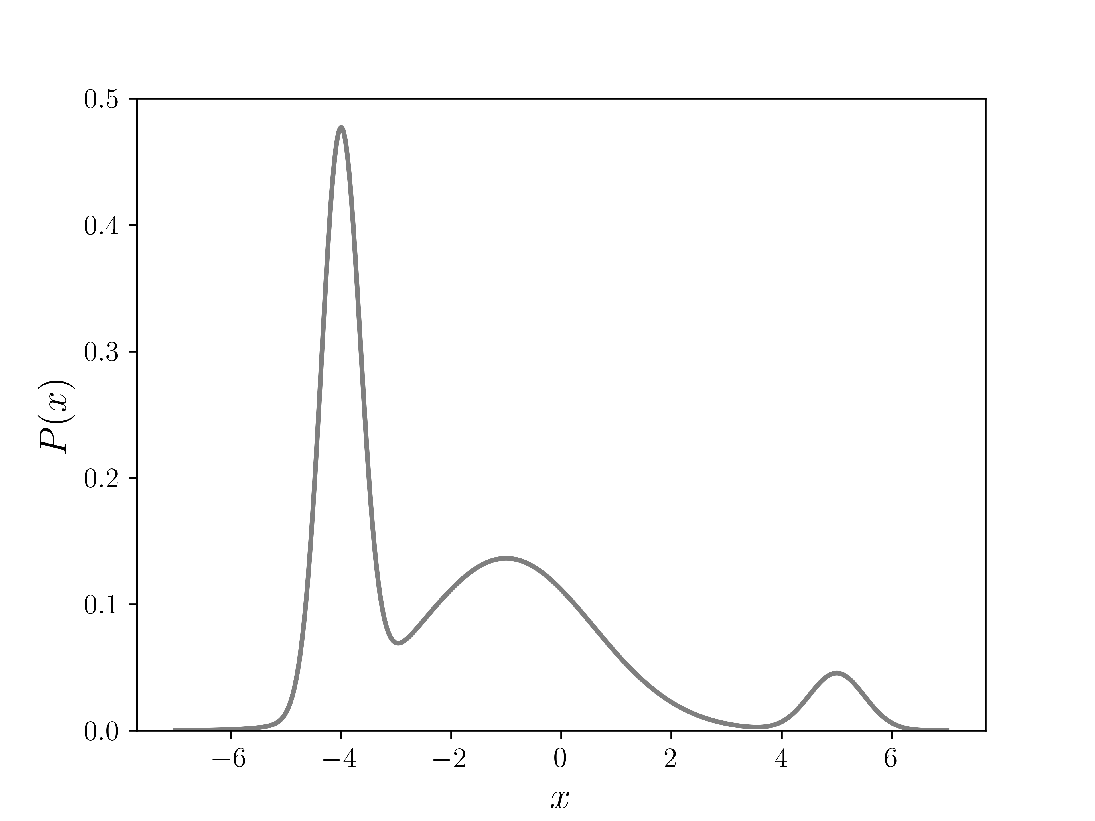
Let our target distribution be $P(x) = \frac{f(x)}{\int_{-10}^{10} f(x)},$

where $f(x)$ is the same function we have shown above and is given by $f(x) = 10e^{-4(x+4)^2} + 3e^{-0.2(x+1)^2} + e^{-2(x-5)^2}.$

The code for defining this function is given below.

def f(x, normalize=False):
    '''
    Function proportional to target distribution, a sum of Gaussians.
    For testing, set normalize to True, to get target distribution exactly.
    '''
    # Gaussian heights, width parameters, and mean positions respectively:
    a = np.array([10., 3., 1.]).reshape(3, 1)
    b = np.array([ 4., 0.2, 2.]).reshape(3, 1)
    xs = np.array([-4., -1., 5.]).reshape(3, 1)

    if normalize:
        norm = (np.sqrt(np.pi) * (a / np.sqrt(b))).sum()
        a /= norm

    return (a * np.exp(-b * (x - xs)**2)).sum(axis=0)

Since this is an easy function to integrate, and hence get our target distribution $P(x)$ directly, we can use it to verify the Metropolis algorithm. The plot of $P(x)$ in the figure below shows three different peaks of varying width and height, with some overlap as well.

Next, we define our walker's symmetric step generating function. As in the random walk example, we will use a random real number between $-1$ and $+1$ as the step size.

def g():
    '''Random step vector.'''
    return np.random.uniform(-1,1)

However, $g$ can be any function symmetric about $0$ for the above algorithm to work. For example, it can be a number chosen randomly from a discrete list, such as $[ -3, -1, -1, +1, +1, +3]$ . It can also be a number chosen from a symmetric continuous distribution, like the Gaussian, $e^{-x^2}$ . In higher dimensions, the function should be spherically symmetric, such as a multidimensional Gaussian function, $e^{-(x^2 +y^2 + ...)}$ . Whatever function you choose, there are at least a couple of things to note:

If the function $g$ is discrete, you will only sample discrete values. For example, if $g$ returns only $-1$ or $+1$ , and nothing in between, you will sample only integer steps away from the initial $x_0$ .
The average step size really matters! A small step-size means the walker will carefully sample nearby regions more, but will walk more slowly, so might not be good at exploring far and wide. On the other hand, a walker with a large step size may not sample nearby regions accurately – and actually has a higher chance of being rejected if the walker is already in a high probability region, since the acceptance ratio is more drastic for large steps. The effect of step-size on the walker's efficiency is far from obvious!

The question of how to choose an optimal $g$ is a research area on its own, and depends largely on what the goal of the sampling is. Some techniques even use an "adaptive" method where $g$ is "trained" on-the-fly using a learning algorithm! Some of these methods and others are discussed in Ref. [8] and Ref. [9]. In a lot of cases, people just use trial and error, as the algorithm is not too difficult to implement.

After choosing $g$ , we are almost ready to iterate. We just need to choose the domain of $x$ , and an initial point for $x_0$ ( $x_t$ at $t = 0$ ) chosen randomly from the domain of $x$ .

xmin, xmax = -10, 10
x0 = np.random.uniform(xmin, xmax)

How to Iterate

Generate new proposed position $x' = x_t + g$ .
Calculate the acceptance probability, $A = \min\left(1, \frac{f(x')}{f(x_t)}\right).$
Accept proposal, with probability . If your programming language doesn't have a built-in method for this,
- Generate a random number $u$ between $0$ and $1$ .
- If $u \leq A$ , then accept move, and set new position, $x_{t+1} = x'$ .
- Otherwise, reject move, and set new position to current position, $x_{t+1} = x_t$ .
Increment $t \rightarrow t + 1$ and repeat from step 1.

The code for steps 1 to 3 is:

def metropolis_iterate(x0, num_steps):
    '''Iterate metropolis algorithm for num_steps using iniital position x_0'''

    for n in range(num_steps):
        if n == 0:
            x = x0
        else:
            x = metropolis_step(x)
        yield x

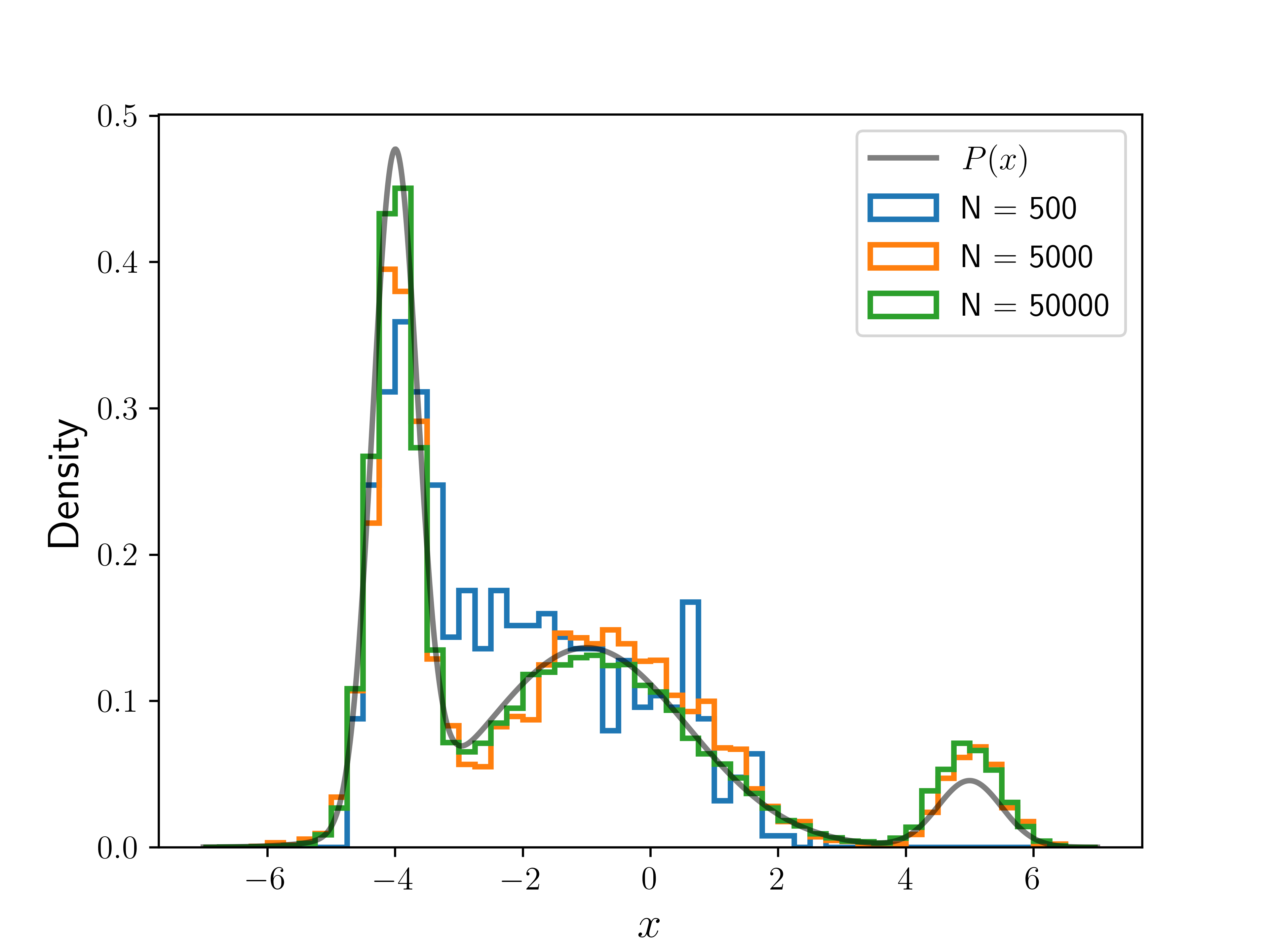
The following plot shows the result of running the algorithm for different numbers of iterations ( $N$ ), with the same initial position. The histograms are normalized so that they integrate to $1$ . We can see the convergence toward $P(x)$ as we increase $N$ .

Example Code

The following code puts everything together, and runs the Metropolis algorithm for a number of steps given by num_steps. All the positions visited by the algorithm are then written to a file, which can be later read and fed into a histogram or other density calculating scheme. The code also incorporates a few tests of the algorithm using the test_metropolis_iterate method. This test will create a normalized density histogram from the generated data, and compare it to $P(x)$ using the Root Mean Square Deviations metric [10].

import numpy as np


def f(x, normalize=False):
    '''
    Function proportional to target distribution, a sum of Gaussians.
    For testing, set normalize to True, to get target distribution exactly.
    '''
    # Gaussian heights, width parameters, and mean positions respectively:
    a = np.array([10., 3., 1.]).reshape(3, 1)
    b = np.array([ 4., 0.2, 2.]).reshape(3, 1)
    xs = np.array([-4., -1., 5.]).reshape(3, 1)

    if normalize:
        norm = (np.sqrt(np.pi) * (a / np.sqrt(b))).sum()
        a /= norm

    return (a * np.exp(-b * (x - xs)**2)).sum(axis=0)

def g():
    '''Random step vector.'''
    return np.random.uniform(-1,1)

def metropolis_step(x, f=f, g=g):
    '''Perform one full iteration and return new position.'''

    x_proposed = x + g()
    a = min(1, (f(x_proposed) / f(x)).item())

    x_new = np.random.choice([x_proposed, x], p=[a, 1-a])

    return x_new

def metropolis_iterate(x0, num_steps):
    '''Iterate metropolis algorithm for num_steps using iniital position x_0'''

    for n in range(num_steps):
        if n == 0:
            x = x0
        else:
            x = metropolis_step(x)
        yield x


def test_metropolis_iterate(num_steps, xmin, xmax, x0):
    '''
    Calculate error in normalized density histogram of data  
    generated by metropolis_iterate() by using 
    normalized-root-mean-square-deviation metric. 
    '''

    bin_width = 0.25
    bins = np.arange(xmin, xmax + bin_width/2, bin_width)
    centers = np.arange(xmin + bin_width/2, xmax, bin_width)

    true_values = f(centers, normalize=True)
    mean_value = np.mean(true_values - min(true_values))

    x_dat = list(metropolis_iterate(x0, num_steps))
    heights, _ = np.histogram(x_dat, bins=bins, density=True)

    nmsd = np.average((heights - true_values)**2 / mean_value)
    nrmsd = np.sqrt(nmsd)

    return nrmsd



if __name__ == "__main__":
    xmin, xmax = -10, 10
    x0 = np.random.uniform(xmin, xmax)

    num_steps = 50_000

    x_dat = list(metropolis_iterate(x0, 50_000))

    # Write data to file
    output_string = "\n".join(str(x) for x in x_dat)

    with open("output.dat", "w") as out:
        out.write(output_string)
        out.write("\n")


    # Testing
    print(f"Testing with x0 = {x0:5.2f}")
    print(f"{'num_steps':>10s} {'NRMSD':10s}")
    for num_steps in (500, 5_000, 50_000):
        nrmsd = test_metropolis_iterate(num_steps, xmin, xmax, x0)
        print(f"{num_steps:10d} {nrmsd:5.1%}")